Introduction to bowerbird
2021-11-22
bowerbird_vignette.rmdbowerbird
A single-cell package for Functional Annotation + Gene Module Summarization.

Bowerbirds are famous for the elaborate and sometimes whimsical structures that males build to court females.
Picture credits: A satin bowerbird’s bower, decorated with blue objects. © Stefan Marks / Flickr
I’m not sure if this mating ritual is in anyway similar to my attempts to visualise pathway analyses and their association with celltype identities/states… who cares. It’s just a name.
Installation
# because currently private, requires specifying personal github access token
devtools::install_github('clatworthylab/bowerbird', auth_token = "insert_your_personal_github_access_token")
# or clone this repo and do devtools::install('path/of/folder/to/bowerbird')
Quick Usage
Pathway analyis is tricky; often there’s too many pathways/terms to use and it’s not easy to distinguish how important every element is. bowerbird attempts to summarise your pathways of interest into potentially meaningful functional annotation modules which you can then take forward to pathway analyses, or the reverse situation where you have a set of pathways that were determined a priori to be significant and you wanted to find out how to interpret it. To do this, we compute a shortest nearest neighbor graph using the genes in the gene sets/pathways and learn a representative summary term from the name of the gene sets that cluster together.
library(bowerbird)
bwr <- bower(gmt_file)
bwr <- snn_graph(bwr)
bwr <- find_clusters(bwr)
bwr <- summarize_clusters(bwr)
bwr <- enrich_genesets(sce, bwr)
Full example
library(bowerbird)
gmt_file <- system.file("extdata", "h.all.v7.4.symbols.gmt", package = "bowerbird") # read in a .gmt file
bwr <- bower(gmt_file) # this performs a read_geneset step internally, which accepts .gmt, .gmx, .csv, .tsv, .txt, or R objects as list or data.frame format.
bwr <- snn_graph(bwr)
bwr <- find_clusters(bwr)
bwr <- summarize_clusters(bwr)
Input formats accepts .gmt, .gmx, .csv, .tsv, .txt, or R objects as list or data.frame format.
csv_file <- system.file("extdata", "h.all.v7.4.symbols.csv", package = "bowerbird") # read in a .gmt file
csv <- read.csv(csv_file)
# see first 6 rows of the first 3 columns
csv[1:6, 1:3]
#>   HALLMARK_ADIPOGENESIS HALLMARK_ALLOGRAFT_REJECTION HALLMARK_ANDROGEN_RESPONSE
#> 1                 ABCA1                        AARS1                      ABCC4
#> 2                 ABCB8                        ABCE1                      ABHD2
#> 3                 ACAA2                         ABI1                      ACSL3
#> 4                 ACADL                         ACHE                      ACTN1
#> 5                 ACADM                       ACVR2A                    ADAMTS1
#> 6                 ACADS                         AKT1                      ADRM1
And now to process it through.
bwr <- bower(csv)
bwr <- snn_graph(bwr)
bwr <- find_clusters(bwr)
bwr <- summarize_clusters(bwr)
Examples of different ways of loading in genesets
Doing some manual editing of a predefined geneset.
# download from msigdb website
file <- system.file("extdata", "c5.go.bp.v7.4.symbols.gmt", package = "bowerbird")
# manualy read in to do some fine adjustments/filtering
geneset <- read_geneset(file) # reads in gene file manually
# do a bit of manual filtering
geneset <- geneset[grep('_B_CELL|_T_CELL|NATURAL_KILLER|ANTIBODY|ANTIGEN|LYMPHOCYTE|IMMUNE|INTERFERON|TOLL|INNATE_IMM|ADAPTIVE_IMM', names(geneset))]

bwr <- bower(geneset)
bwr <- snn_graph(bwr)
bwr <- find_clusters(bwr)
bwr <- summarize_clusters(bwr)
Or extracting from msigdbr.
library(msigdbr)
GO <- data.frame(msigdbr::msigdbr(category = "C5", subcategory = "GO:BP"))
genesets <- GO[grep('_B_CELL|_T_CELL|NATURAL_KILLER|ANTIBODY|ANTIGEN|LYMPHOCYTE|IMMUNE|INTERFERON|TOLL|INNATE_IMM|ADAPTIVE_IMM', GO$gs_name), ]

# convert to list
gs_list <- lapply(unique(genesets$gs_name), function(x) genesets[genesets$gs_name %in% x, "gene_symbol"])
names(gs_list) <- unique(genesets$gs_name)

bwr <- bower(gs_list)
bwr <- snn_graph(bwr)
bwr <- find_clusters(bwr)
bwr <- summarize_clusters(bwr)
So what has actually happened? Well, basically bowerbird has learnt which gene sets share more genes with each other, clustered them together and learnt a new summary term.
bwr
#> BOWER class
#> number of genesets:  254
#> genesets kNN Graph:
#> IGRAPH bd2602e UNW- 254 799 --
#> + attr: name (v/c), cluster (v/n), geneset_size (v/n), terms (v/c),
#> | labels (v/c), weight (e/n)
#> + edges from bd2602e (vertex names):
#> [1] GOBP_ACTIVATED_T_CELL_PROLIFERATION--GOBP_CD8_POSITIVE_ALPHA_BETA_T_CELL_DIFFERENTIATION
#> [2] GOBP_ACTIVATED_T_CELL_PROLIFERATION--GOBP_NEGATIVE_REGULATION_OF_ACTIVATED_T_CELL_PROLIFERATION
#> [3] GOBP_ACTIVATED_T_CELL_PROLIFERATION--GOBP_NEGATIVE_REGULATION_OF_LYMPHOCYTE_DIFFERENTIATION
#> [4] GOBP_ACTIVATED_T_CELL_PROLIFERATION--GOBP_NEGATIVE_REGULATION_OF_T_CELL_RECEPTOR_SIGNALING_PATHWAY
#> [5] GOBP_ACTIVATION_OF_IMMUNE_RESPONSE --GOBP_ACTIVATION_OF_INNATE_IMMUNE_RESPONSE
#> + ... omitted several edges
#> number of geneset clusters:  21
#> Core genes:
#>  First six genes shown
#>   IMMUNE RESPONSE-1 : AIM2 BCL10 BTRC CARD11 CARD9 CD209 ...
#>   CD4 ALPHA BETA T CELL DIFFERENTIATION : ANXA1 ATP7A BATF BCL3 BCL6 CBFB ...
#>   IMMUNE RESPONSE : CLNK HLA-E HLA-F IFNA2 IFNB1 IL18 ...
#>   T CELL MEDIATED CYTOTOXICITY : HLA-A HLA-B HLA-C HLA-E HLA-F HLA-G ...
#>   CD8 ALPHA BETA T CELL ACTIVATION : HLA-E GATA3 ADCYAP1 BTK C3 CCR7 ...
#>   B CELL PROLIFERATION : ADA BAX BCL6 BLK BTK CD74 ...
#>   B CELL DIFFERENTIATION : CAMP DEFA1 DEFA1B DEFA3 DEFA4 DEFA5 ...
#>   T CELL DIFFERENTIATION : FCGR2B FGL2 HLA-DOA LILRB2 THBS1 BMP4 ...
#>   INTERFERON GAMMA PRODUCTION : ABCB9 ACE ACTR10 ACTR1A ACTR1B AP1B1 ...
#>   T HELPER 1 TYPE IMMUNE RESPONSE : IFNB1 IL4 IL6 TBX21 BCL6 FOXP3 ...
#>   TOLL LIKE RECEPTOR SIGNALING PATHWAY : CACTIN PTPRS TICAM1 TLR3 TLR4 TLR9 ...
#>   T CELL CYTOKINE PRODUCTION : KLRC1 LILRB1 NOD2 PTPRC EGR3 LEF1 ...
#>   RESPONSE TO INTERFERON BETA : ADA SOS1 SOS2 IRF1 TLR3 IRGM ...
#>   T CELL SELECTION : TOX BCL2 BATF CTSL FOXP3 IL12B ...
#>   B CELL ACTIVATION : ADA ADAM17 BATF BCL3 BCL6 BTK ...
#>   ACTIVATED T CELL PROLIFERATION : LILRB4 CD24 CD274 FYN HHLA2 ICOSLG ...
#>   LYMPHOCYTE CHEMOTAXIS : CCL2 CCL3 CCL4 CCL5 CCL7 CXCL14 ...
#>   INFLAMMATORY RESPONSE TO ANTIGENIC STIMULUS : BTK C3 CD28 HLA-E LTA NOD2 ...
#>   ALPHA BETA T CELL ACTIVATION : AGER ANXA1 ARG2 ATP7A BATF BCL3 ...
#>   LYMPHOCYTE MIGRATION : ADAM10 ADAM17 ADAM8 AIF1 APP CCL20 ...
#>   ANTIGEN PROCESSING AND PRESENTATION OF PEPTIDE ANTIGEN VIA MHC CLASS I : ABCB9 AZGP1 B2M ERAP1 ERAP2 HFE ...
We can visualise it with a simple plot
plot_graph(bwr, colorby = 'cluster', node.size = 'geneset_size')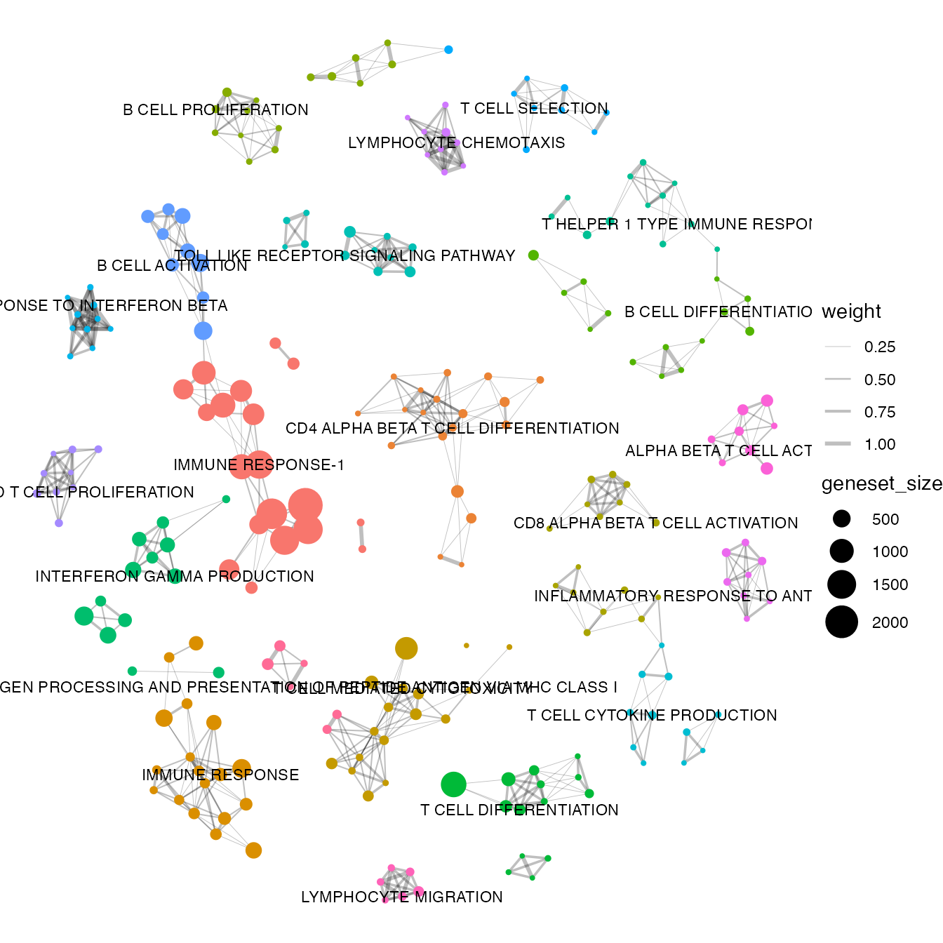
Geneset average expression testing
We can also compute the enrichment score and superimpose the values onto the visualization. To do this, we would need either a single-cell object (SingleCellExperiment or Seurat), or a list containing differential gene testing results.
With popular single-cell methods.
## AUCell
bwr <- enrich_genesets(kidneyimmune, bwr, groupby = 'celltype', mode = 'AUCell')

## Seurat::AddModuleScore
bwr <- enrich_genesets(kidneyimmune, bwr, groupby = 'celltype', mode = 'Seurat')

## scanpy.tl.score_genes
bwr <- enrich_genesets(kidneyimmune, bwr, groupby = 'celltype', mode = 'scanpy')
Visualise as a network plot.
celltypes <- levels(kidneyimmune) # celtypes stored as Idents in seurat object.
plot_list <- lapply(celltypes, function(ds){
  g <- plot_graph(bwr, colorby = ds) + viridis::scale_color_viridis() + theme(plot.title = element_text(size = 8, face = "bold"))
})
cowplot::plot_grid(plotlist = plot_list, scale = 0.9)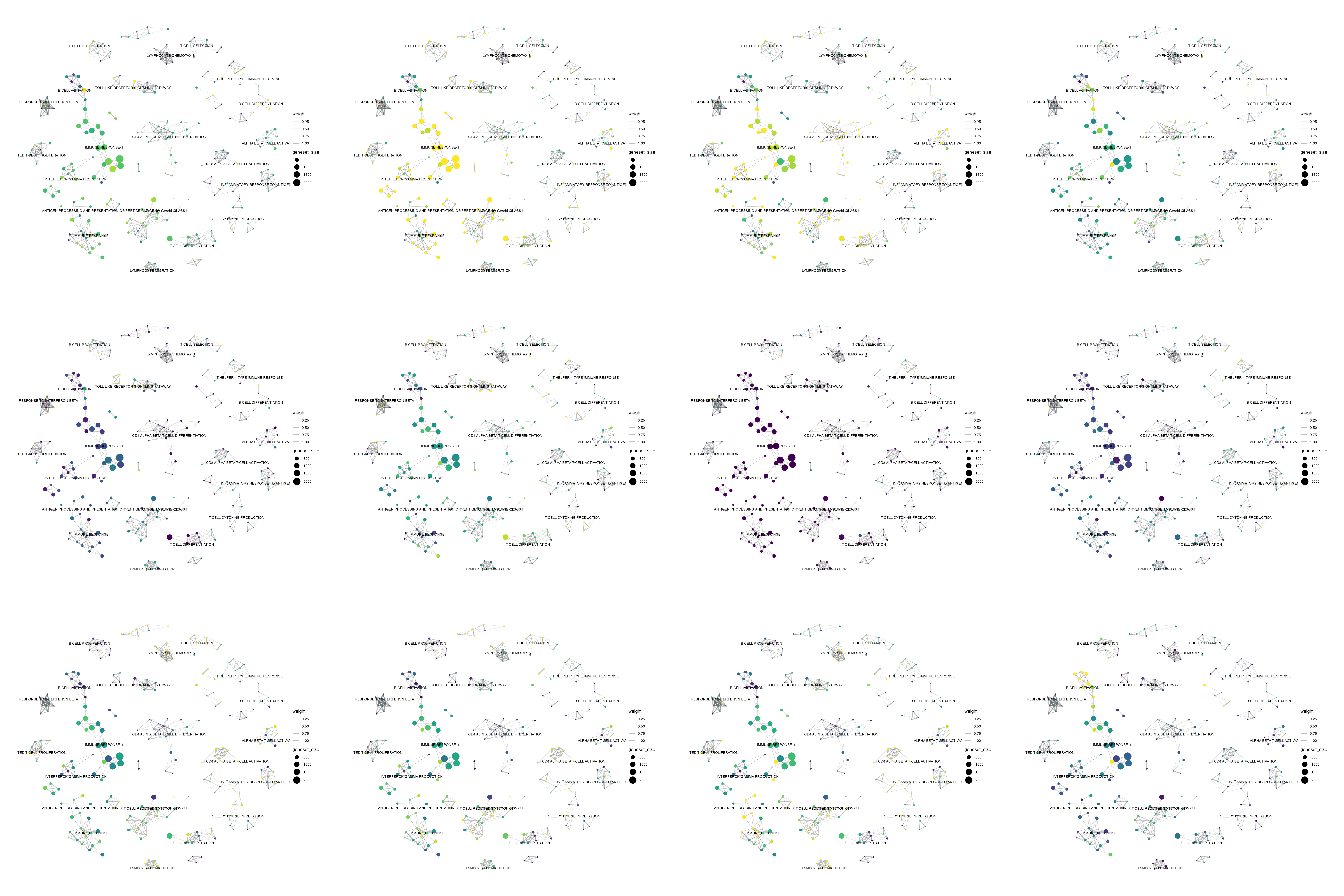
Running fgsea on deg tables in a list as an alternative to the single-cell methods.
Here we use a differential expression result for marker genes as input.
degs <- Seurat::FindAllMarkers(kidneyimmune)
degs <- split(degs, degs$cluster) # so in practice, there should be one DEG table per comparison in a list.
bwr <- enrich_genesets(degs, bwr, gene_symbol = 'gene', logfoldchanges = 'avg_log2FC',  pvals = 'p_val')
Coloured by adjusted p value.
plot_list <- lapply(celltypes, function(ds){
  g <- plot_graph(bwr, colorby = ds, mode = 'gsea', gsea.slot = 'padj') + viridis::scale_color_viridis(na.value = '#e7e7e7') + theme(legend.position = 'none', plot.title = element_text(size = 8, face = "bold"))
})
cowplot::plot_grid(plotlist = plot_list, scale = 0.9)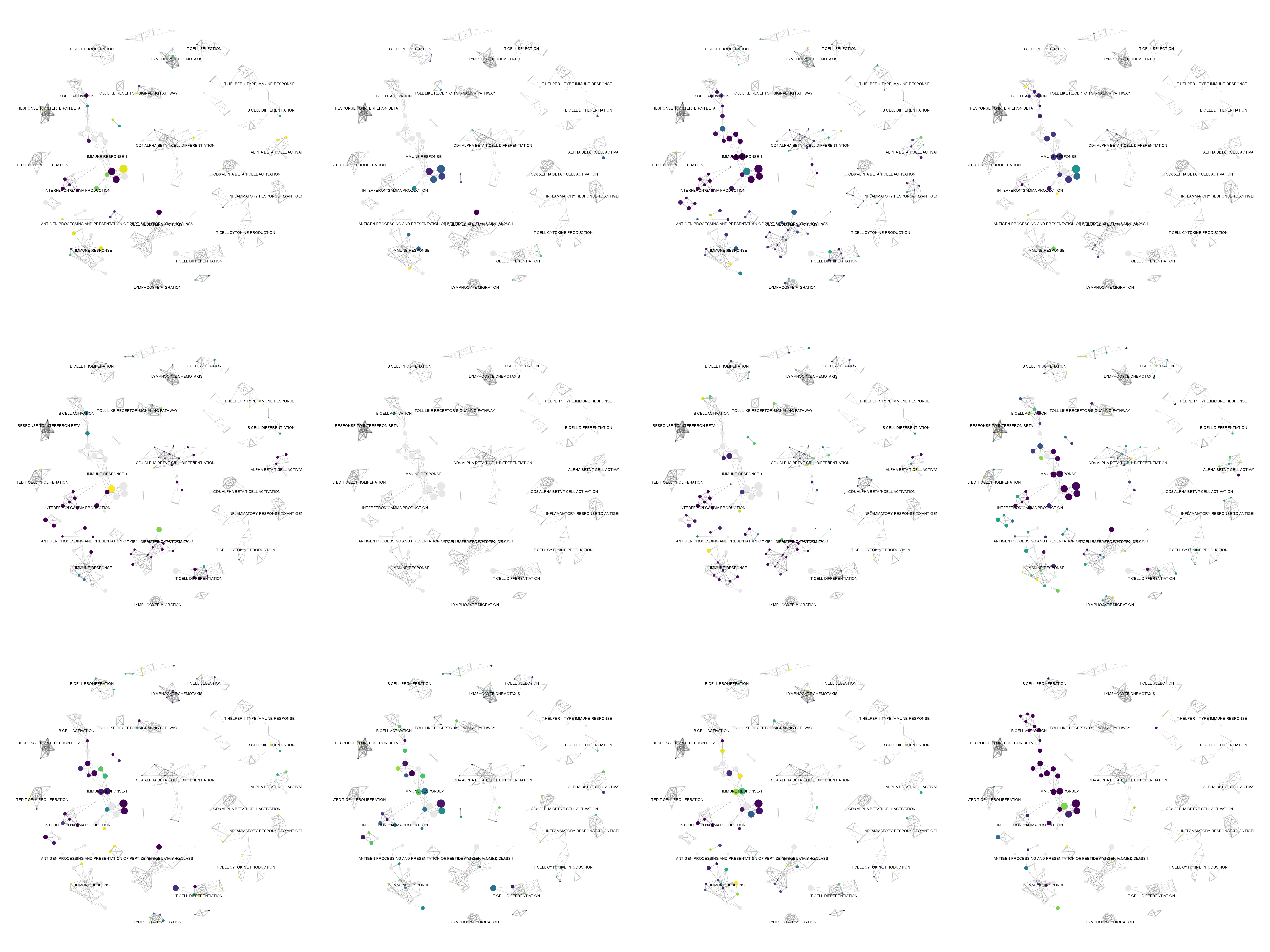
Coloured by normalized enrichment score.
plot_list <- lapply(celltypes, function(ds){
  g <- plot_graph(bwr, colorby = ds, mode = 'gsea', gsea.slot = 'NES') + viridis::scale_color_viridis(na.value = '#e7e7e7') + theme(legend.position = 'none', plot.title = element_text(size = 8, face = "bold"))
})
cowplot::plot_grid(plotlist = plot_list, scale = 0.9)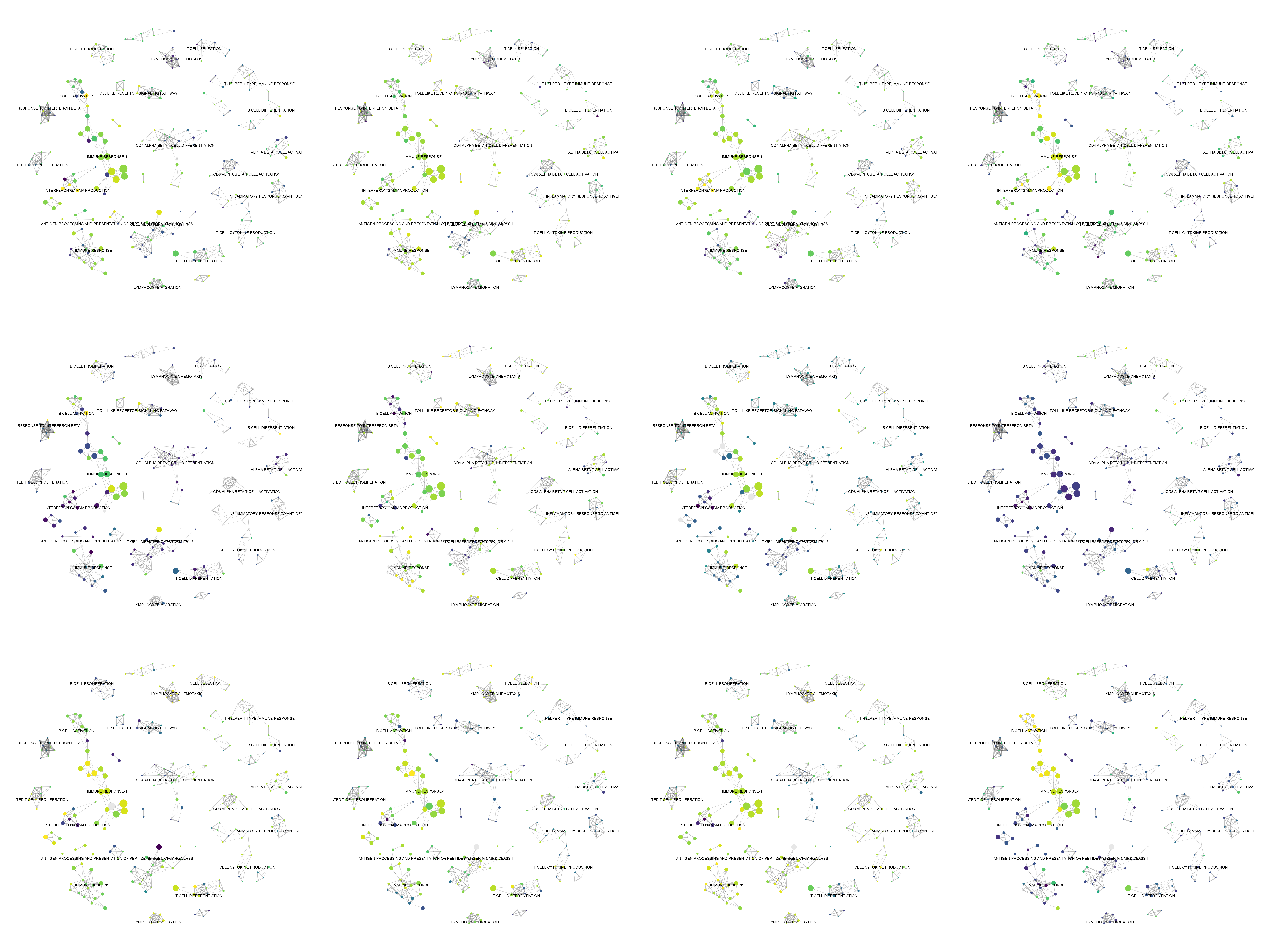
Using core genes for enrichment
Same function as above, just specifying core = TRUE. This will grab the intersecting (or outersecting rather) genes in a gene set cluster and perform the enrichment, like a summary gene set of the summarised terms.
bwr <- enrich_genesets(kidneyimmune, bwr, core = TRUE, groupby = 'celltype') # if mode is not specified, the default option is to use AUCell
pheatmap::pheatmap(bwr@scores, cellheight = 20, cellwidth = 20)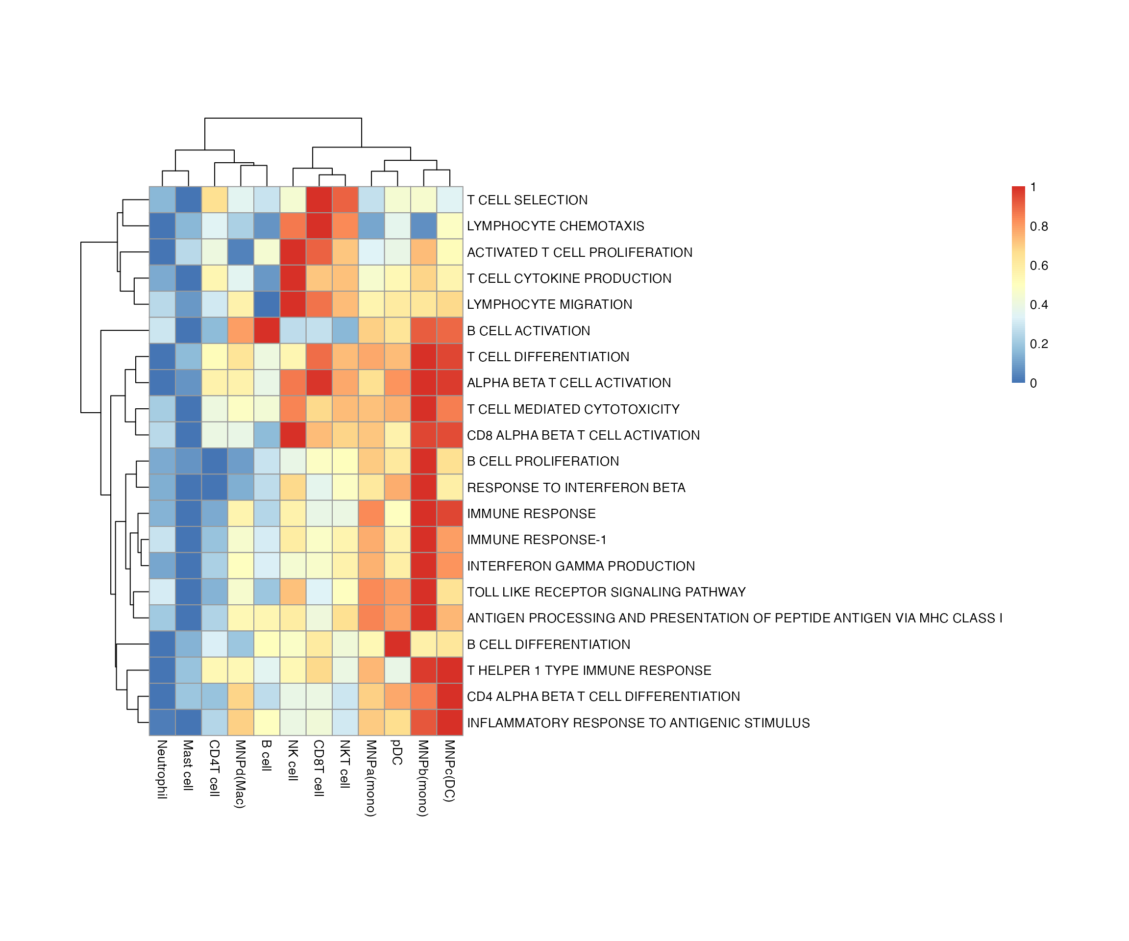
Same for the gsea results. First looking at the NES.
bwr <- enrich_genesets(degs, bwr, core = TRUE, gene_symbol = 'gene', logfoldchanges = 'avg_log2FC',  pvals = 'p_val')
pheatmap::pheatmap(bwr@scores$NES, cellheight = 20, cellwidth = 20)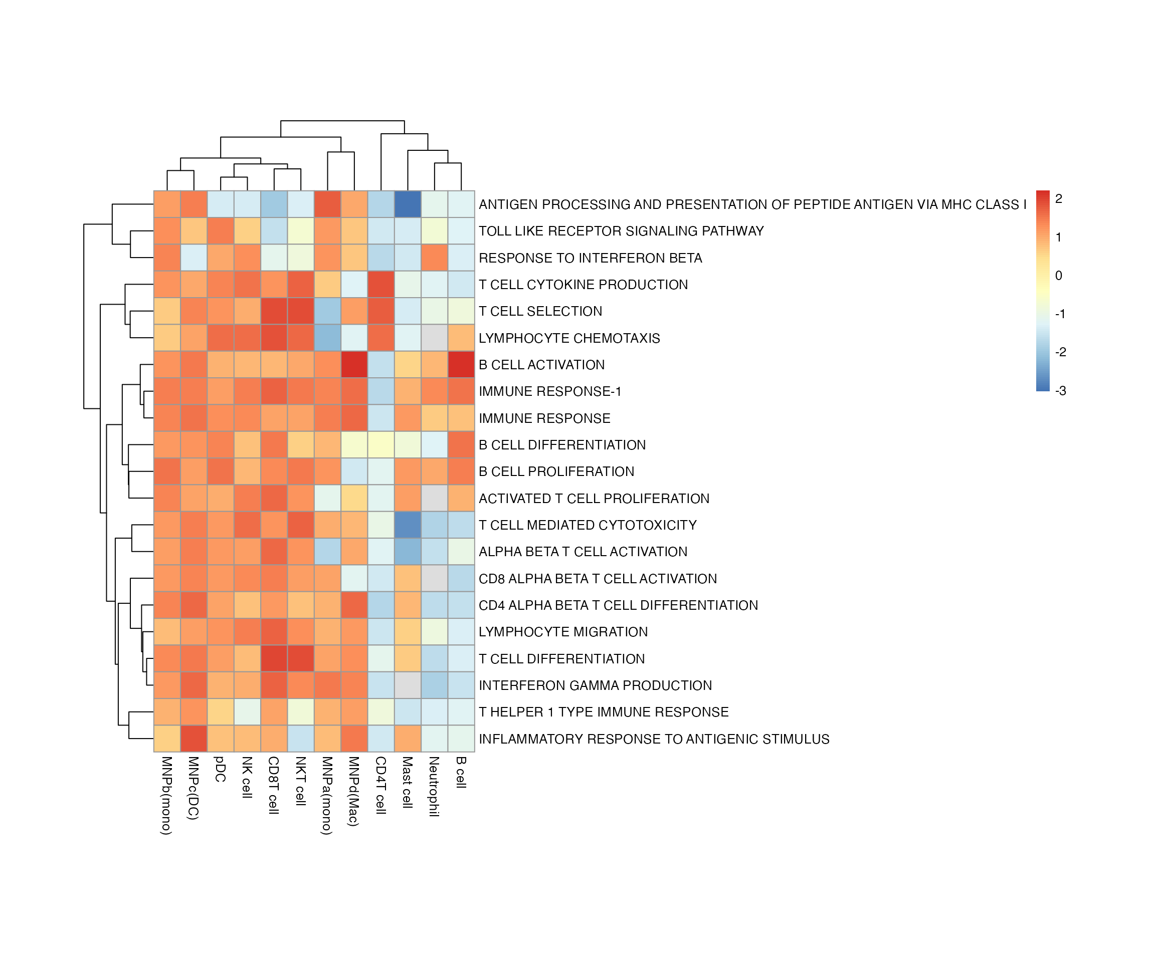
And now the FDR, remembering that <0.25 is usually the cut off.
pheatmap::pheatmap(bwr@scores$padj, cellheight = 20, cellwidth = 20, color = viridis::viridis(50, direction = -1))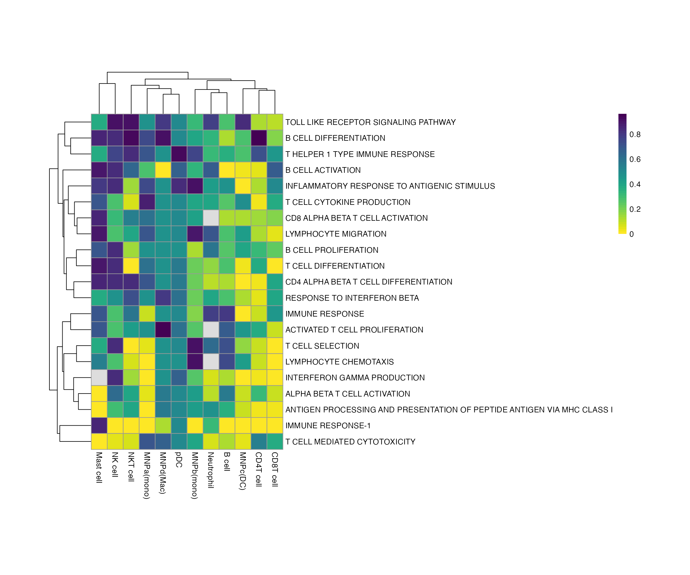
To visualise as a graph, can consider doing:
bwr2 <- bower(bwr@coregenes)
# and so on
Hopefully you find this interesting and potentially useful.
Please email me at kt16@sanger.ac.uk if you have any queries, feedback or ideas and I’ll get back to you!
